Taking the L2HMC Sampler for a "Spin"

Introduction

Finding sampling algorithms that can efficiently cover ill-conditioned distributions is a difficult challenge, even for popular methods such as Hamiltonian Monte Carlo. Recently, the L2HMC method demonstrated low autocorrelation and high expected sample size over various ill-conditioned energy landscapes (Levy et al. 2018). By training deep neural networks to maximize the expected squared jump distance, the MCMC kernel can more efficiently explore the distribution. While promising, the initial training time of their sampler is not accounted for and could pose problems in practice when applying L2HMC to new distributions. In this project, I set out to analyze the training time and performance of different neural networks on strongly correlated gaussian distributions. I also examine whether one L2HMC sampler can be used to sample from multiple similar distributions.

Background

Hamiltonian Monte Carlo

Hamiltonian Monte Carlo (HMC) is a type of Markov Chain Monte Carlo (MCMC) algorithm where new states are proposed through Hamiltonian dynamics (Neal 2012). Given that we can write our target distribution as a function of an energy distribution $p(x) \propto \exp(-U(x))$, we can approximate hamiltonian dynamics to explore this distribution using a series of leapfrog updates as follows: \begin{equation} v^{\frac{1}{2}} = v - \frac{\epsilon}{2}\partial_x U(x); \quad x’ = x+\epsilon v^{\frac{1}{2}}; \quad v’ =v-\frac{\epsilon}{2} \partial_x U(x’). \end{equation}

L2HMC Algorithm

The Learning to Hamiltonian Monte Carlo (L2HMC) algorithm modifies the HMC dynamics using trained neural networks (Levy et al. 2018). The usual leapfrog update steps are modified by scaling functions S,Q,T. The function S scales the current position or momentum, the function Q scales the derivative, and the function T translates the new position or momentum vector. Levy et al. showed that these dynamics have tractible determinants of the jacobian and preserves the properties of a markov chain, while efficiently exploring the distribution it was trained on.

The way the sampler increases its efficiency is by training these dynamics functions to maximize the expected squared jump distance. The expected squared jump distance from one state vector $\xi$ can be written in the form of equation below. \begin{equation} ESJD := \sum_{\xi’} P(\xi’|\xi)\lVert \xi_x-\xi_x’ \rVert_2^2 \end{equation}

Here $\xi_x$ denotes the position subcomponent of the full state vector.

The standard architecture for each network of the L2HMC sampler (for position and momentum updates) used by Levy et al. is defined as follows: Position, velocity, and time step of the sampler serve as the input variables. This input is sent through two fully connected (ReLU activation) layers using hidden layer width of 10 for most energy functions, and 100 for the 50-dimensional ill conditioned gaussian (ICG). The output from this step is fed separately into the final translation/scaling layers, S,Q,T. The networks were trained for 5,000 iterations.

Experimental Setup

The L2HMC repository from Levy et al. was forked and modified for the current project. Tests were run on Google Colab Pro with a Tesla P100 PCI-E GPU, Intel Xeon Processor, and 13 Gb of RAM.

Network Width

We first analyze how changing the width of the network affects both training and performance of the L2HMC sampler. We run 2500 training iterations of 200 L2HMC chains (this is effectively the batch size) for fully connected neural networks of hidden layer widths 5, 10, and 20. Loss and acceptance history, as well as total training time was recorded. Once the sampler is fully trained, auto-correlation and expected sample size (ESS) is also measured, again using 200 chains simualted for 2000 time steps. For the sake of time we limit our analysis to the 2-dimensional strongly correlated gaussian (SCG) from Levy et al., with variances along the eigenvectors of $10^2$ and $10^{-1}$.

Rotational Invariance

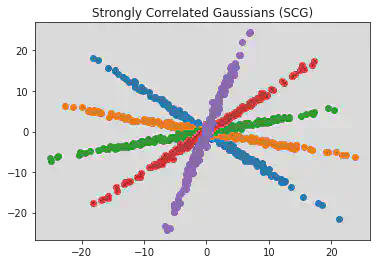
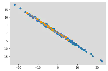
Next we look at how well one L2HMC sampler can adapt to distributions similar to the one it was trained on. Ideally, one would like to train one sampler to perform well on an entire class of distributions, as opposed to retraining each time. While there are many ways one distribution can be similar to another, in this project we focus on rotations of the same distribution. For our tests we use the SCG distribution whose covariance matrix is rotated by a certain degree. An example of this rotation is provided in figure 1.

We first determine how well a sampler trained on our original SCG performs on rotated distributions of increasing degree. By estimating at what point the sampler’s performance drops off, we can get a sense of its “operational range”. Most likely the limits determined here in the low dimensional setting upper bound those in the high dimensional setting, as many small differences in angle would result in large overall distances between distributions.

We finally make an attempt to train our sampler on multiple distributions in an effort to further generalize its performance. After a certain number training iterations we swap out the energy function of our sampler, switching between 5 SCG’s each rotated by 30 degrees. We also try a less extreme augmentations, switching between 5 SCG’s rotated by a smaller degree. We first measure our performance on one of the training distributions, and then a new test distribution (still within the training rotation range).

Results

Network Width

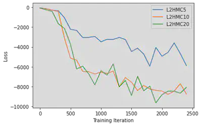
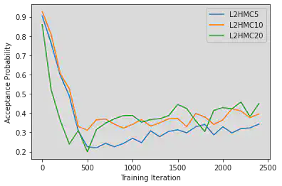
We first provide comparisons of our training and performance data for different network sizes. In figure 2, one can see that the loss for networks size 10 and 20 seem to plateau at around -8,000, while the smaller network of size 5 seems to have not yet reached a minima. While harder to interpret than something like the MSE loss (which is at best 0), our version of the expected squared jump distance loss can be roughly lower bounded in our toy example by bounding the maximum “width” of our distribution (more robustly one might consider something like gaussian complexity or a concentration bound on the difference between two independent samples from our distribution). We note that as our expected squared jump distance grows larger the second term in equation \ref{eq:loss} dominates. \begin{equation} \label{eq:loss} \ell_{\lambda} (\xi, \xi’, A(\xi’|\xi)) = \frac{\lambda^2}{\delta(\xi,\xi’)A(\xi,\xi’)} -\frac{\delta(\xi,\xi’)A(\xi,\xi’)}{\lambda^2} \end{equation} If we consider coordinates (-20,20) to (20,-20) to be the “endpoints” of our distribution measurement, and using a scale parameter of $\lambda^2 = 0.1$, we can bound our loss as: \begin{equation} \ell_{\lambda} \geq -\frac{40^2+40^2}{0.1} = -32,000 \end{equation} This lower bound seems to align with empirical results. We can further check whether our sampler’s are well trained by monitoring the acceptance probability. While in general this is not the case, we know that for a low dimensional gaussian distribution our acceptance probability should be around 44% \cite{}.In figure 3, we see the samplers appear to be converging to exactly that, again with the 5-width network trailing behind the other two samplers.

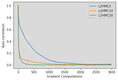
Next we compare the fully trained sampler performances. Looking at figure figure 4, we see that both 10-width and 20-width networks have almost negligible autocorrelation within a hundred gradient computations (10 samples), while the 5-width sampler takes an order of magnitude more (100 samples) to reach the same level. This performance gap is reflected in the ESS as well, with the 20-width sampler beating the 5-width by a factor of 10, and the 10-width by a factor of 2. Interestingly, both training and sampling times are roughly comparable between all three samplers. This may be because of the slight variation in allocated resources of the Google Colab platform, but is most likely a result of the lower dimensional problem setting. One might expect that for higher dimensional problems changes in network width would result in many more computations per training iteration. Most important to note however is that training time takes an order of magnitude longer than sample time (for approximately the same number of iterations). This means that one can’t ignore training time when calculating ESS per time unless the number of samples being considered is much larger than what it takes to train the sampler. Even worse, since this training time most likely grows with the complexity of the distribution (while the number of samples needed remains relatively constant) the training time factor may begin to dominate when calculting total ESS per time.

Network Size	Training Time (s)	Sample Time (s)	ESS
5	651	69	1.48e-02
10	597	61.5	9.13e-02
20	595	61.4	2.09e-01

Rotational Operating Range

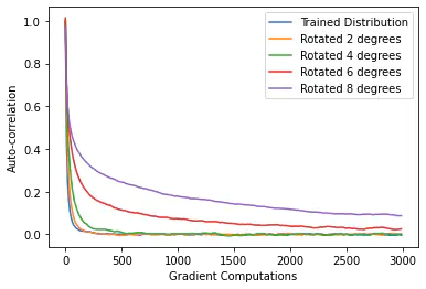
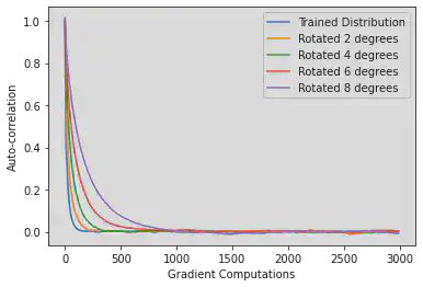
We see in figure 5 that the basic 10-width L2HMC sampler has a relatively narrow range of good performance. Any time the training distribution is rotated by more than 8 degrees, autocorrelation remains high until around 100 samples later. This performance drop-off is also seen in the ESS, which at 8 degrees is smaller by a factor of 10, and by plotting a MCMC chain for this distribution (figure 6). We see that the chain is having a harder time reaching the extremes of this rotated distribution.

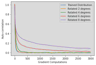
As we increase the width and expressivity of our network, we see our operating range actually decreases (figure 7). The autocorrelation of the width-20 sampler tested on the 8 degree rotated distribution is much worse than earlier, and is still not negligible after 300 samples. We include in table 2 the full list of expected sample size of samplers tested on the rotated distributions, where we see this trend continues.

Network Size	ESS (trained)	ESS (2deg)	ESS (4deg)	ESS (6 deg)	ESS (8deg)
10	2.99e-01	1.58e-01	9.24e-02	5.26e-02	3.07e-02
20	3.15e-01	2.31e-01	1.17e-01	2.60e-02	7.31e-03
40	3.07e-01	4.89e-02	7.34e-03	3.13e-04	2.64e-04

This means that although we demonstrated previously that the width 10 and 20 samplers had similar performance on the training distribution, the larger width sampler is less robust to variations in the distribution, indicating possible overfitting. It may therefore be worthwhile to attempt to train the smallest network that gives good performance on the training distribution to improve expected sample size in practice.

An interesting future line of work would be to examine whether this rotational sensitivity also depends on how strongly correlated the distribution is. One could imagine in the trivial case of a perfectly spherical gaussian distribution that rotations would leave the covariance matrix unchanged, and hence the 2lhmc sampler would perform just as efficiently.
Regardless, we can conclude from this experiment that the base L2HMC sampler is probably “memorizing” the energy function it was trained on, rather than learning a general set of dynamics for strongly correlated distributions.

Conclusion

In this work we have shown that training time of the L2HMC algorithm cannot be considered negligible when the number of samples needed is on the same order as the number of training iterations. We have also observed a key trade-off of the sampler between maximizing performance on the training distribution and maximizing its robustness to rotations. Lastly we have illustrated the limitations of the base L2HMC sampler when trying to generalize performance to an entire class of distributions. Future work is needed to determine whether this limitation can be overcome through better network architecture (an engineering issue) or whether it is inherent to the algorithm (in which case a new algorithm is needed).